Vortex Shedding
I have been working on my Lattice-Boltzmann simulation code recently. (Okay, given how long this article has been a draft, ‘recently’ is perhaps a stretch.) Simulating the vortex shedding of flow past a cylinder is practically a rite-of-passage for CFD codes. So let’s do it!
All the results shown here were produced with my code, which is available on GitHub.
Specifically the script at vortex_street.py.
Contents
Setup
Flow Geometry
The flow setup (shown in the diagram) is a rectangular domain of height \(W\) and length \(L\). At the left and right ends in- and out-flow boundaries are enforced by prescribing that the velocity be equal to \(\mathbf u = (u, 0)\). The top and bottom boundaries are periodic. In the (vertical) centre of the domain is a circular wall boundary of diameter \(D\). Let’s define the y-axis such that \(y=0\) corresponds to the midline of our simulation.

This setup is called flow past a cylinder because we imagine the 2D simulation is a slice of a 3D system which is symmetric under translations in the z-direction.
Characteristic Scales
The suitable characteristic length-scale is the diameter of the cylinder \(D\), and the characteristic velocity is the prescribed in-flow velocity \(u\). Combined with the fluid’s kinematic viscosity - \(\nu\) - these give us the Reynold’s number
$$\mathrm{Re} = \frac{uD}{\nu}$$The flow displays different behaviour depending on the value of \(\mathrm{Re}\). We can control this by changing any of \(u\), \(D\) or \(\nu\). In the simulations below I have done this by fixing \(D\) and \(\nu\) then inferring \(u\).
The characteristic timescale of the system is the time it takes the fluid to flow past the cylinder
$$T = \frac{D}{u}$$We define the ‘dimensionless time’ to be \(\tau = t/T\). When comparing results across different Reynold’s numbers we will plot them at equal values of dimensionless time.
Because our simulation domain is finite in size we, strictly, also have to consider the dimensionless ratio \(D/W\); the ‘obstruction’. However we will sweep that under the table for now.
Flow Regimes
Depending on the Reynold’s number this setup displays 4 distinct behaviours.
| Re. | Behaviour |
|---|---|
| <10 | Creeping |
| 10 - 100 | Recirculation |
| 100 - 1000 | Vortex Shedding |
| > 1000 | Turbulence |
These ranges are only approximate. I have seen various figures quoted in different sources, for instance sometimes it’s stated that shedding starts at around Re = 40. In my results Re = 50 was stable for the whole simulation, unless I manually induced shedding by perturbing the initial velocity field.
Simulation
Initial Conditions
When setting up the simulation we could set the initial velocity to be equal to \(u\) everywhere. However, directly up- & downstream of the cylinder the velocities will be pointing respectively into, and out-of the wall boundary. This means, at these points, the velocity field is not divergence free.
At low velocities this causes a large “sound” wave to propagate outwards from the cylinder (compression at the leading edge and rarefaction at the trailing edge.) The velocities induced by this can be of similar order to the flow features we’re interested in. They will eventually propagate out of the domain but it’s needlessly ugly.
Here is what the initial disturbance looks likes for \(Re = 100:\)

The compression/rarefaction seen here is larger than 4%!
More problematically, at higher velocities (Reynold’s numbers) these pressure waves can even cause the simulation to become unstable and blow up. We have to do something better!
Stream Function
The initial pressure waves are mostly caused by the non-zero divergence of the velocity field. Therefore we can naturally think to start with a velocity field that is divergence free.
There are a few approaches we could try to get such initial conditions. One such is to construct a stream function, and to use this to get the velocity field. This works because stream functions exist only for divergence free flow fields, thus any velocity field derived from a stream function is guaranteed to be divergence free.
The stream function is a 2D scalar field - \(\psi\) - whose derivatives in each direction specify the velocity vector:
$$u_x = \frac{\partial \psi}{\partial y} \qquad u_y = -\frac{\partial \psi}{\partial x}$$Because the velocity is specified by the gradients of \(\psi,\) it is not unique; any constant offset will yield the same velocity field.
A uniform velocity field $(u, 0)$, corresponds to stream functions of the form \(\psi_\text{uniform} = u y + C.\) Wlog. choose \(C = 0,\) so that the stream function is zero along the mid-line of our simulation. Next, we can notice that if the stream function’s gradients are zero at the cylinder walls then we have zero velocity here. Thus if we perturb \(\psi_\text{uniform}\) near the wall s.t. this is the case, we will get a velocity field which has the desired value far from the cylinder, tends to zero near the cylinder and is divergence free. Nice!
Obviously the stream function \(\psi = 0\) has zero gradient everywhere, and conveniently matches \(uy\) on the midline. So we can imagine interpolating between \(\psi = 0\) near the wall and \(\psi = uy\) far from the wall:
$$\psi = f(d)\cdot uy + \cancel{(1-f(d)) \cdot 0}$$where \(d\) is the distance from the solid wall.
The interpolation function must have the following properties:
- \(f(\infty) = 1\) - One far from the walls.
- \(f(0) = 0\) - Zero near the walls.
- \(f^\prime(0) = 0\) - Zero gradient near the walls.
The last property is required because otherwise we would get a non-zero x-velocity at the wall:
$$u_x = \frac{\partial \psi}{\partial y}\bigg|_{d=0} = uy \partial_y f(0) + f(0)u$$An obvious candidate is
$$f(d) = 1-e^{-(d/D)^2}$$because \(e^{-x^2}\) has zero gradient at the origin. Moreover the gradient is actually linear around zero, which matches the expected velocity profile near a wall (see Wikipedia.)
If we plug in \(f\) we can evaluate the exact form of \(u_x\) along the vertical line extending from the cylinder. We find that there is a region (\(d > \sqrt{D/2}\)) where \(u_x > u\). This makes sense physically. We need the overall flow rate to remain constant (mass conservation), so we must have a higher velocity region to compensate the zero velocity near the wall and the channel width reduction due to the cylinder.
Distance Function
To use calculate the stream function above we need to know the distance to our cylinder - \(d.\) This is very simple to calculate using the signed distance function for a circle. However, we can keep it more general by using the Euclidean distance transform. This lets us perform the same calculations for arbitrary geometries.
Here is an example of the stream function initial conditions applied to a semi-circular boundary:

Putting this together gives us the divergence free initial conditions for our simulation. The updated simulation start-up is shown below, with the same colour-scale as above:

The density fluctuations are much reduced, showing a maximum compression/rarefaction of under 1%. More importantly the simulation remains stable for higher Reynold’s numbers.
Density Initial Conditions
But why do we still see any density fluctuations? Ultimately it’s because the Lattice-Boltzmann method (LBM) solves for approximately incompressible flows.
In an incompressible fluid the pressure acts to keep the flow exactly divergence free. Fluid in the LBM is slightly compressible, with the pressure being related to the density via the equation of state
$$P = \rho c_s^2$$But the flow is still almost incompressible so we expect corresponding pressure gradients, and these pressure gradients imply density gradients via the equation of state. Therefore, even without the initial transients, we will always see some density fluctuations in our LBM simulations.
We can use Bernoulli’s principle and the equation of state to relate the density to the velocity as
$$\frac{\rho}{\rho_0} = 1 - \frac{v^2 - u^2}{2c_s^2} \label{density_bernoulli}\tag{1}$$Where I have used the fact that all streamlines in our initial velocity field end at the in-flow boundary, letting us fix the constant in Bernoulli’s relation. \(\rho_0\) is the arbitrary density at the in-flow.
We can use equation \eqref{density_bernoulli} to set the initial condition for the density. Even doing this, however, we would still expect some initial transients. This is because the stream function we used is arbitrary (up to the constraints), and is not a solution to the Navier-Stokes equation (probably).
Surprisingly, I found that setting the initial density in this way actually made the transients marginally worse. Therefore, for my simulations I have simply let the density be uniform throughout the domain.
Plotting
Choosing Colour-scales
In order to accurately compare the results across different Reynold’s numbers it is important for the colour-scales to match. All the results shown here have a velocity magnitude colour-scale from 0 to \(2u\), and a vorticity colour-scale from \(-50u/D\) to \(+50u/D.\) These numerical prefactors were determined empirically to give useable scales.
Streamlines
When visualizing flow fields the streamlines can be a useful addition, even for time varying flows. One difficulty with plotting them, is choosing the seed points from which to integrate the velocity field. For example, if we choose some seed points at the inflow boundary, then we will not see any streamlines in the recirculation regions behind the cylinder. To get around this we can actually make use of the stream function again.
The contours of the stream function correspond to the stream lines of the velocity field. Therefore if we calculate the stream function, we can easily plot streamlines including in disconnected parts of the flow. (This is going the other way from the initial conditions where we went from the stream function to the velocity.)
One definition of the stream function is that it is the flux through any path from a reference point to the current position. This is given by the line integral
$$\psi(\mathbf x) = \int_{\mathbf x_\mathrm{ref}}^{\mathbf x} \mathbf v \cdot \hat{\mathbf n} \,dl$$Because the exact path is not important we can arbitrarily say we will take a path which goes first vertically, and then horizontally from \(\mathbf x_\mathrm{ref}\) to \(\mathbf x.\) Thus the integral becomes
$$\psi(\mathbf x) = \int_{y_\mathrm{ref}}^y v_x dy + \int_{x_\mathrm{ref}}^x v_y dx$$which is something we can easily calculate numerically.
It is important to note that although \(\mathbf x_{\mathrm{ref}}\) does not affect the velocity field we would get back from the \(\psi\), it obviously affects the value of \(\psi\) itself. We need our contour levels to be consistent over time, so we need to choose a reference point whose velocity does not change. I have used the lower-left corner, which is in the inflow boundary and thus has velocity fixed at \(u.\)
Results
This section shows the results of the simulation for various Reynold’s numbers, at a late dimensionless time \(\tau=100.\) This is enough time to let the initialization effects fully propagate out of the domain, and for the flow to establish its long-time behaviour. The chosen Reynold’s numbers display the four regimes mentioned above; creeping flow, recirculation, vortex shedding and, finally, turbulence.
The simulations for Reynold’s number 5 and 50 have domains with grid sizes 1000 × 3000, i.e. 3 million cells. The higher Reynold’s numbers require a higher resolution and so were run at 4000 × 12,000, i.e. 48 million cells.
If you’re interested in seeing the time evolution you can head over to YouTube, for a video showing the simulation for Re = 500 and Re = 5000. Re = 5 and Re = 50 are not worth a video since they settle into a steady-state!
I have not embedded the video here, primarily, because of the cookie implications. But also because, unasked, YouTube has decided the video is a “Short”, which affects the embedding.
Cylinder Frame
First, let’s look at the fluid velocity (magnitude) in the rest frame of the cylinder. This is how the simulation is actually run, and matches the set-up described above with in- and out-flow boundary conditions.

We can see, as expected, the four flow regimes for the different Reynold’s numbers.
For Re \(<\) 100 we see that, after the initial transients have advected out of the domain, the flow settles into a steady-state with no vortex shedding. In both cases there is a region of “stagnant” flow trapped just behind the cylinder, which has zero net velocity.
For Re = 50, if we look closely, we can see a slight non-zero velocity along the midline in the middle of this stagnant region. In fact, the velocity is not only non-zero, it is heading in the direction opposite to the bulk flow! This is because the flow is recirculating. It’s hard to see when looking at the whole domain and with the chosen colour scale, though, so let’s look a zoom of just the recirculation region.
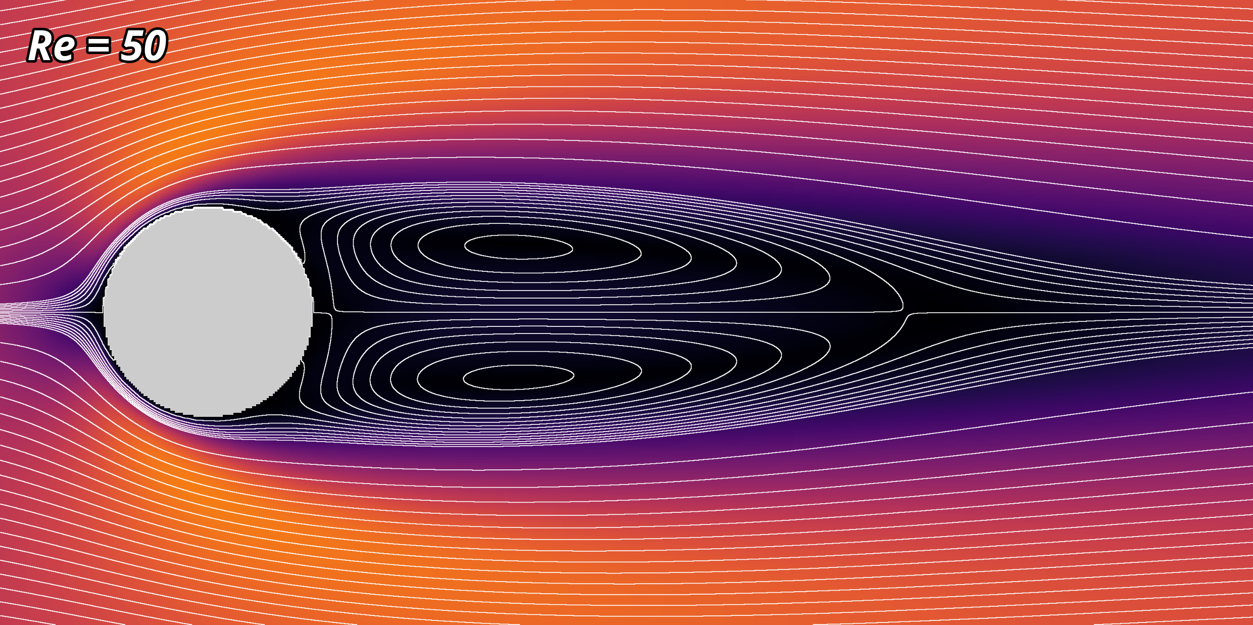
Here I have not blended the streamlines with the velocity field, as above, but just overlain them directly to make them more visible. Because the simulation is steady-state for Re = 50, the streamlines do correspond to pathlines of the flow, and we see that just downwind of the cylinder they are closed loops. This means that fluid is trapped, and being pushed around in a vortex motion, i.e it is recirculating.
At higher Reynold’s numbers the recirculation zone grows, and eventually becomes unstable. First one of the recirculation vortices is shed, then while it reforms the the other is shed, etc. When looking at the plot for Re = 500 above, however, it is not obvious that the periodic flow feature behind the cylinder is a sequence of vortices. The flow is not steady-state, so the streamlines do not correspond to path- or streaklines of the flow. Despite that, the fact they are not closed here doesn’t make them look much like a vortices. This can be remedied by considering the fluid’s own rest-frame.
Fluid Frame
Instead of considering the cylinder fixed, and the fluid as flowing past it with velocity \(u\), we could equally well consider the fluid as being fixed and the cylinder moving through it with velocity \(-u.\) This is the ‘fluid frame’. The fluid frame velocity is given by \(v_x^\prime = v_x - u\) and \(v^\prime_y = v_y,\) and the magnitude is correspondingly changed.

In this frame we see that for Re = 5 and Re = 50, the stagnant region behind the cylinder is, instead, an entrained pocket of fluid. For the fluid rest frame the streamlines do not coincide with the pathlines even for Re = 5 and Re = 50, because in this frame cylinder is viewed as moving, therefore the flow cannot be steady-state.
For Re = 500 and Re = 5000, despite the flow also not being-steady state, the streamlines do form closed loops behind the cylinder, showing that we have formed vortices.
At Reynold’s number 500 they form a regular line, with each vortex rotating in the opposite sense to its neighbours. The vortices are not moving relative to the surrounding fluid, the non-zero velocity in this reference frame purely shows their rotation. Although it is tempting to think it looks like the entrained fluid pocket for lower Reynold’s numbers, it is not. The high velocity in the band behind the cylinder is actually perpendicular to the cylinders motion. Picture the cylinder moving through stationary fluid, leaving a line of vortices, whose centers are stationary, in its wake.
By the time we get to Re = 5000, turbulence has set in and they shoot off in random directions, and tend to form pairs of oppositely rotating vortices. If you watch the video, you can even see that these sometimes collide and the pairs swap vortices.
From the velocity magnitude + streamlines we cannot tell which way the vortices are rotating. This, we can visualize with the vorticity.
Vorticity
The vorticity is given by the curl of the velocity field: \(\nabla\times\mathbf v.\) It is unchanged by a constant offset of the velocity
$$\boldsymbol{\omega}^\prime = \nabla\times\mathbf v^\prime = \nabla\times(\mathbf v + \mathbf u) =\nabla\times\mathbf v + \nabla\times\mathbf u = \nabla\times\mathbf v = \boldsymbol{\omega}$$because for a constant vector \(\nabla\times\mathbf u = 0.\) Therefore, it does not matter if we take the curl of the cylinder-frame or the fluid-frame velocity field.

Orange shows positive vorticity (i.e. anticlockwise rotation) and blue, negative vorticity (clockwise rotation).
Mechanisms
Creeping Flow
At very low Reynold’s numbers, creeping flow shows neither time evolution, nor eddies. In this regime the flow is governed by Stokes equations, which does not have any time dependence. Its inertia is so weak compared to viscosity, that it instantly responds everywhere to the boundary conditions.
Recirculation
For slightly higher Reynold’s numbers the approximation behind Stokes flow, that viscosity completely dominates inertia, starts to break down and we do get eddies forming.
These are formed behind the cylinder by flow separation. As the fluid flows past the cylinder it is at first constricted, which means the velocity must increase (mass conservation) and thus the pressure decreases (Bernoulli’s principle). Once past the midpoint, however, the channel becomes less constricted again and the velocity drops, and thus the pressure increases. The overall flow is therefore going against the pressure gradient at this point. Near the boundary the flow is slower, so this adverse pressure gradient actually causes the flow here to reverse, and go against the bulk flow, causing the eddies.
An obvious question to ask is why is the recirculation stable for these intermediate Reynold’s numbers? Why do we not see vortices being shed here? Unfortunately I could not find a good answer in the literature. (One must exist, surely?)
If I were to hazard a guess I’d say that, although we now have recirculating eddies, the flow is still viscous enough that the bulk behaves more-or-less like Stokes flow. Disturbances in the flow are felt quickly far away via the rapid diffusion of momentum associated with the high viscosity. The bulk flows around the combined “cylinder + eddies” obstacle, which “deconstricts” more gently than the cylinder alone, thereby ameliorating the adverse pressure gradient for the bulk. (One obvious feature of this interpretation is that, although the cylinder has no-slip boundary conditions, the eddies most certainly do not. But perhaps that does not matter.)
Shedding
I think the exact cause of the vortex shedding is not currently well understood. At least, that’s what’s stated in the abstract of nearly every paper I looked at whilst trying to understand the mechanism(s) involved in vortex shedding. Many papers investigating vortex shedding are numerical, rather than theoretical, and examine simulations in fine detail. While useful, I was looking for something more mathematical.
I found this paper by Boghosian & Cassel quite nice; it is at the same time sufficiently mathematical and quite readable. It examines under which situations vortices in 2D incompressible flow split. The gist of the paper is that at points of zero momentum, having \(\nabla\cdot\frac{d\mathbf u}{dt} > 0\) will cause a vortex to split. While I like the paper, I don’t think it explains the vortex shedding mechanism observed here. They show that for a general vortex the pressure gradient is not enough to get the divergent net force, so they need to add a body force. That is clearly not the situation we have here.
A common suggestion for the cause of vortex shedding, which seems sensible to me, is a form of Kelvin-Helmoltz instability.
The fluid-frame velocity magnitude plots for Re = 50 show how we have two shear layers just downstream of the cylinder; one extending from the top, and one from the bottom. This is true in the early flow for higher Reynolds numbers too. Because of the Kelvin-Helmholtz instability, this shear layer is unstable and will naturally form growing vortices.
This makes sense but it cannot be the whole story; the shear layer exists also for lower Reynold’s numbers, and according to theory, shear layers are always unstable (if the densities of the fluid on either side are equal.) This is the flip-side of the question of why the recirculating vortices are stable for low Re; why do they become unstable for higher values of Re?
von Kármán Vortex Street
But wait, what about the famous von Kármán Vortex Street? This is the famous effect whereby vortices shed behind an obstacle create two rows of opposite rotational sense, between which the vortices are offset from one another. This is beautifully illustrated in this satellite image from NASA:

Consider two rows of vortices separated by a distance denoted \(h\), with each row containing vortices rotating in opposite directions. Within each row let the distance between vortices be denoted by \(l\). According to von Kármán’s analysis, any arrangement apart from \(\frac{h}{l} = \frac{1}{\pi}\mathrm{arcosh}(\sqrt{2})\approx0.28\) is unstable.
His original paper from 1911* (in German) can be found here, and an English translation of his second paper*, also from 1911, is available here. It is quite readable and I suggest that the interested reader give it a look.
However, my simulations did not show this predicted, and rather beautiful, pattern. Instead, the vortices form a single line of alternating sense along the midline. Why?
I think the answer, ultimately, comes down to boundary conditions. I ran the simulations with a larger domain and I do see the predicted offset vortices:

The vortices have been visualized here by letting two tracers (dyes) advect with the fluid; the top half of the obstacle releases red dye, and the bottom green. Where these mix it creates yellow, but you can clearly see the red & green dye trapped in the vortices being carried off downstream.
To Make the tracers more visible downstream I have boosted the contrast between zero- and low tracer concentrations, by updating values to be \(\sqrt C.\)
This simulation was run at Re = 100. In the simulations I ran, at lower Reynold’s number the von Kármán pattern developed closer to the obstacle. For higher Reynold’s numbers it did develop, just somewhat downstream of the obstacle. However, with the original shorter geometry, even at Re = 100 the vortices formed a line, rather than the von Kármán pattern.
Consider the velocity field formed by the vortex street arrangement, in the rest frame of the bulk fluid. I will describe it with words, but to aid the subsequent description, let’s just look at it:

Between neighbouring pairs of opposite sense vortices the fluid flows fast, and on the outer edges of the vortices, slowly. Thus fluid between the two rows is, on average, moved to the left (for our configuration). The vortices themselves “roll” between this moving central fluid, and the stationary bulk fluid. This rolling causes some slight rightward motion of the bulk fluid just outside the vortex street.
If we imagine averaging the fluid’s velocity over time we get the right-hand side of the above figure. This clearly shows how the fluid behind the cylinder is entrained and has non-zero velocity.
This is the reason, then, I believe the boundary conditions are affecting the vortex street formation. For the vortex street, the velocity profile along a vertical slice is anything but uniform and steady-state. By contrast, our boundary conditions set a uniform and constant velocity across the whole right-hand edge.
Because the vortex street has a leftward velocity relative to the velocity at our boundary, it is forced to accelerate as it exits the domain. This has the effect of pulling the vortices inwards. Additionally (and perhaps more importantly?) the constant velocity outflow condition kills any rotational motion as the flow approaches the boundary.
This suggests an interesting test would be to implement some more sophisticated boundary conditions, e.g. non-reflecting / characteristic boundary conditions, which will let the vortices flow out of the system unimpeded.
References
- On the Origins of Vortex Shedding in Two-dimensional Incompressible Flows - M. E. Boghosian & K. W. Cassel (link)
- Über den Mechanismus des Widerstandes, den ein bewegter Körper in einer Flüssigkeit erfährt - Theodore von Kármán (link)
- On the mechanism of the drag a moving body experiences in a fluid - Theodore von Kármán (link)